🏍️ Modelling Riders Performance

Key findings and achievements

• For the purpose of providing more technical insights to fans, we demonstrate how public race data can be used to extract important information on race and rider performance.
• We demonstrate how to quantify the performances of riders, teams, and constructors through quantitative indicators that take into account relative speed and consistency, the two fundamental variables in a theoretical definition of race performance.

---

Introduction

Sports are being radically transformed by data collection and analysis, benefiting both professionals and fans. Soccer, baseball, and American football are some examples where player performance data is utilized to acquire talent and provide in-depth statistics for the public. In contrast, data analysis for motorsports fans is not yet widespread, despite being fundamental to the sport’s operation.

In this notebook, we will explore the realm of MotoGP racing and analyze publicly available race data with the aim of comprehending how it can be used to provide fans with essential insights on riders’ performance. By employing statistical methodologies, we will extract as much insights as possible from the openly accessible data, contending that it is possible to gauge the riders’ objective performances within a race and across the championship. At the same time, we will propose potential data analyses – presented as a “post-GP” information product – that can be used by the media to interpret Grand Prix outcomes and which can spark engaging discussions on the competitors’ performance levels and progress.

Data is provided thanks to the motogpdata project.

import motogpdata.handler as mgphandler
import pandas as pd
import seaborn as sns
import matplotlib.pyplot as plt

Race Results

For the scope of this study, we will take into account and examine two races from the 2022 MotoGP season, namely the Qatar Grand Prix and the Italian Grand Prix. Let’s first refresh our memory of the results of these races.

For the Qatar Grand Prix:

season = mgphandler.Season(2022, 'MotoGP')
qat2022 = mgphandler.Event(season, 'QAT')
ita2022 = mgphandler.Event(season, 'ITA')

results_subset = ['rider.full_name', 'position', 'average_speed', 'total_laps', 'time', 'points']
qat2022.results()[results_subset].set_index('rider.full_name')

	position	average_speed	total_laps	time	points
rider.full_name
Enea Bastianini	1.0	168.2	22	42:13.1980	25
Brad Binder	2.0	168.1	22	42:13.5440	20
Pol Espargaro	3.0	168.1	22	42:14.5490	16
Aleix Espargaro	4.0	168.0	22	42:15.4400	13
Marc Marquez	5.0	167.9	22	42:17.2970	11
Joan Mir	6.0	167.8	22	42:18.0410	10
Alex Rins	7.0	167.6	22	42:22.0080	9
Johann Zarco	8.0	167.5	22	42:23.7340	8
Fabio Quartararo	9.0	167.5	22	42:23.7410	7
Takaaki Nakagami	10.0	167.2	22	42:28.1650	6
Franco Morbidelli	11.0	167.1	22	42:29.9100	5
Maverick Viñales	12.0	166.6	22	42:36.4140	4
Luca Marini	13.0	166.4	22	42:40.4810	3
Andrea Dovizioso	14.0	166.4	22	42:40.5720	2
Remy Gardner	15.0	165.5	22	42:54.3050	1
Darryn Binder	16.0	165.5	22	42:54.3170	0
Fabio Di Giannantonio	17.0	165.5	22	42:54.5470	0
Raul Fernandez	18.0	165.4	22	42:55.5550	0
Francesco Bagnaia	NaN	167.2	11	21:13.8350	0
Jorge Martin	NaN	167.2	11	21:13.8000	0
Miguel Oliveira	NaN	166.9	10	19:19.8860	0
Alex Marquez	NaN	166.6	9	17:25.7820	0
Jack Miller	NaN	165.4	6	11:42.3060	0
Marco Bezzecchi	NaN	165.6	6	11:41.3210	0

For the Italian Grand Prix:

ita2022.results()[results_subset].set_index('rider.full_name')

	position	average_speed	total_laps	time	points
rider.full_name
Francesco Bagnaia	1.0	175.1	23	41:18.9230	25
Fabio Quartararo	2.0	175.1	23	41:19.5580	20
Aleix Espargaro	3.0	175.0	23	41:20.9060	16
Johann Zarco	4.0	175.0	23	41:21.5130	13
Marco Bezzecchi	5.0	174.9	23	41:21.9900	11
Luca Marini	6.0	174.9	23	41:22.7980	10
Brad Binder	7.0	174.9	23	41:22.9900	9
Takaaki Nakagami	8.0	174.4	23	41:29.8670	8
Miguel Oliveira	9.0	174.3	23	41:30.1790	7
Marc Marquez	10.0	174.3	23	41:30.7230	6
Fabio Di Giannantonio	11.0	174.2	23	41:31.8390	5
Maverick Viñales	12.0	174.2	23	41:31.8400	4
Jorge Martin	13.0	173.9	23	41:36.1630	3
Alex Marquez	14.0	173.9	23	41:36.4910	2
Jack Miller	15.0	173.9	23	41:36.6100	1
Darryn Binder	16.0	173.7	23	41:39.1880	0
Franco Morbidelli	17.0	173.7	23	41:39.2190	0
Michele Pirro	18.0	173.6	23	41:40.2280	0
Remy Gardner	19.0	173.0	23	41:49.4710	0
Andrea Dovizioso	20.0	173.0	23	41:49.9340	0
Raul Fernandez	21.0	172.2	23	42:01.6460	0
Lorenzo Savadori	22.0	164.9	22	41:58.6110	0
Enea Bastianini	NaN	174.8	13	23:24.0940	0
Joan Mir	NaN	172.8	7	12:44.7980	0
Alex Rins	NaN	173.5	7	12:41.6070	0
Pol Espargaro	NaN	171.2	4	07:21.0900	0

The traditional race classification tables (which represent the only type of data considered by most of the media when convering races) do not provide many analytical insights nor objective indicators of riders performances. They merely offer a snapshot of the race outcome; and the final result does not provide a comprehensive evaluation of the competitors’ achievements in the race.

It is in fact possible for a rider to finish a race in a certain position thanks to the mistakes of others, even if he has maintained an anonymous performance throughout the competition. In such situations, the most common question that arises is whether or not the rider “deserved” or not the position he achieved at the end of the race. In other words, we ask: what was the rider’s performance after accounting for the race events? How can we measure and evaluate his performance regardless of the result obtained?

Laptime analysis

A statistical assessment of race performance is required to address these inquiries, which entails an evaluation based on factual data rather than subjective sentiments or judgments. To accomplish this, the data on lap times must be taken into account, scrutinizing the race’s overall progress. An illustration of such data for the Qatar race is presented below.

# Extract race analysis data for the Qatar Grand Prix
timesheetQAT, laptimes_ridersQAT, laptimes_teamsQAT, laptimes_constructorsQAT, performanceQAT = qat2022.race_analysis(save_pdf=False, performance=True)
laptimes_ridersQAT_melted = laptimes_ridersQAT.melt(id_vars='lap', var_name='rider', value_name='laptime')

laptimes_ridersQAT.head()

rider	Aleix Espargaro	Alex Marquez	Alex Rins	Andrea Dovizioso	Brad Binder	Darryn Binder	Enea Bastianini	Fabio Di Giannantonio	Fabio Quartararo	Francesco Bagnaia	...	Marc Marquez	Marco Bezzecchi	Maverick Viñales	Miguel Oliveira	Pol Espargaro	Raul Fernandez	Remy Gardner	Takaaki Nakagami	avg_laptime	lap
lap
1	121.559	122.479	122.363	123.815	121.021	124.531	121.438	125.299	122.042	121.817	...	120.713	122.419	124.207	122.558	120.669	125.229	125.051	122.755	122.863542	1
2	115.237	116.054	115.487	116.887	115.086	116.721	114.953	116.269	115.415	115.135	...	115.265	116.229	116.618	116.259	115.181	116.272	116.173	115.975	115.839625	2
3	114.797	115.223	114.610	115.858	114.846	115.720	114.918	115.982	115.007	114.771	...	114.875	115.636	116.134	115.488	114.797	116.531	115.974	115.909	115.377417	3
4	115.000	115.329	114.706	115.860	115.069	115.591	114.991	116.212	115.171	115.223	...	115.032	116.318	116.044	115.057	115.076	116.106	116.167	116.029	115.478208	4
5	114.944	115.328	115.013	117.290	114.867	116.474	114.956	116.228	115.236	115.105	...	114.867	115.520	116.015	115.097	114.753	116.326	116.210	115.380	115.526708	5

5 rows × 26 columns

The above table (in its comprehensive form) shows the lap times of each rider (expressed in seconds), and provides already a good starting point for deepening the understanding of the time trends and the general race progression. From such data, it is possible to generate some of the following visualizations.

sns.relplot(data=laptimes_ridersQAT_melted[laptimes_ridersQAT_melted['rider'].isin(
    ['avg_laptime', 'Enea Bastianini', 'Aleix Espargaro', 'Raul Fernandez'])], 
            x='lap', y='laptime', hue='rider', kind='line', 
            palette=['green', 'red', 'darkorange', 'grey'], aspect=1.5)

plt.title("Qatar 2022\nComparative Lap Time Analysis - Riders")
plt.xlabel("Laps")
plt.ylabel("Lap times (in seconds)")
plt.show()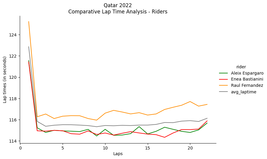

By projecting the average lap time (gray line), we can appreciate the general trend of the race. For example, in the case of Qatar, there is a decline in overall performance starting from the seventeenth lap. Similarly, there is a significant performance drop in the Italian Grand Prix race starting from the sixteenth lap. This analysis helps to evaluate tire performance.

Regarding the personal lap times of the riders, we can notice that both Enea Bastianini (who arrived in 1st place) and Aleix Espargaro (who arrived in 4th place) performed well below the average (gray line), unlike Raul Fernandez, for example (orange line), who consistently raced above the general average of the competition. Similar considerations can also be applied to the Italian Grand Prix, as shown below.

timesheetITA, laptimes_ridersITA, laptimes_teamsITA, laptimes_constructorsITA, performanceITA = ita2022.race_analysis(save_pdf=False, performance=True)
laptimes_ridersITA_melted = laptimes_ridersITA.melt(id_vars='lap', var_name='rider', value_name='laptime')

sns.relplot(data=laptimes_ridersITA_melted[laptimes_ridersITA_melted['rider'].isin(
    ['avg_laptime', 'Francesco Bagnaia', 'Fabio Quartararo', 'Andrea Dovizioso'])], 
            x='lap', y='laptime', hue='rider', kind='line', 
            palette=['aqua', 'blue', 'red', 'grey'], aspect=1.5)

plt.title("Mugello 2022\nComparative Lap Time Analysis - Riders")
plt.xlabel("Laps")
plt.ylabel("Lap times (in seconds)")
plt.show()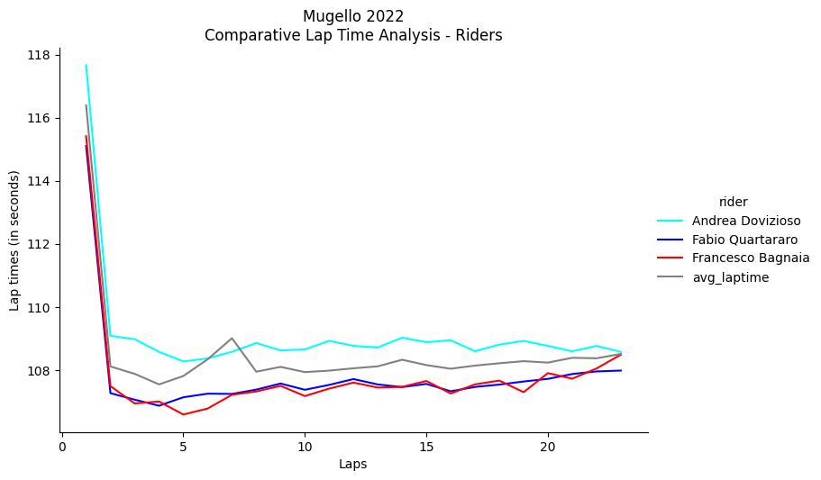

These graphs provide a visual and intuitive way to determine if a particular rider, team, or manufacturer has performed above, below, or at an average level. (It’s important to note that the more a rider’s lap times are below the average race’s lap time, the faster they’ve gone). Using the same visualization concept for the constructors, we can see how Yamaha and KTM consistently performed above average in the Qatar 2022 race, thus indicating that they “underperformed” compared to the other manufacturers.

laptimes_constructorsQAT_melted = laptimes_constructorsQAT.melt(id_vars='lap', var_name='constructor', value_name='laptime')

sns.relplot(data=laptimes_constructorsQAT_melted[laptimes_constructorsQAT_melted['constructor'].isin(
    ['avg_laptime', 'Yamaha', 'KTM'])], 
            x='lap', y='laptime', hue='constructor', kind='line', 
            palette=['darkorange', 'blue', 'grey'], aspect=1.5)

plt.title("Qatar 2022\nComparative Lap Time Analysis - Constructors")
plt.xlabel("Laps")
plt.ylabel("Lap times (in seconds)")
plt.show()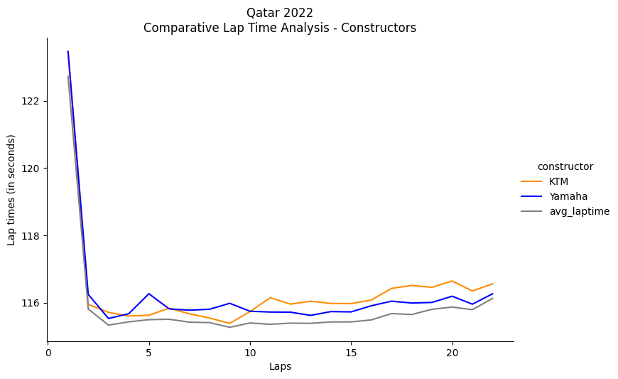

Sector times

In an aggregate manner, it is also possible to determine variation indicators for each sector of the circuit, thereby appreciating the overall level of consistency of the riders in the various sections of the track. For example, we can observe that in the case of the Qatar Grand Prix, the consistency of lap times in different sectors is almost identical, while at Mugello, the sector in which the riders were on average more consistent is T2.

std_race = pd.DataFrame(timesheetQAT[timesheetQAT['lap'] != 1][['t1', 't2', 't3', 't4']].std())
std_race = std_race.pivot_table(columns=std_race.index).round(2)
std_race.index = ['σ']
print("🇶🇦 Qatar Grand Prix 2022\nSector Pace:")
std_race

🇶🇦 Qatar Grand Prix 2022
Sector Pace:

	t1	t2	t3	t4
σ	0.21	0.23	0.21	0.21

std_race = pd.DataFrame(timesheetITA[timesheetITA['lap'] != 1][['t1', 't2', 't3', 't4']].std())
std_race = std_race.pivot_table(columns=std_race.index).round(2)
std_race.index = ['σ']
print("🇮🇹 Italian Grand Prix 2022\nSector pace:")
std_race

🇮🇹 Italian Grand Prix 2022
Sector pace:

	t1	t2	t3	t4
σ	0.46	0.24	0.74	0.45

The same principle of analysis can be applied to the fastest times set by riders in the different sectors of the track. At the Mugello Grand Prix, we can see, for example, how Yamaha, with Fabio Quartararo, was the fastest in T2 and T3. In contrast, the Ducatis of Bagnaia and Bastianini expressed the best times in the sectors with higher top speeds (T1 and T4) due to the long straights.

by_rider = timesheetITA[timesheetITA['lap'] != 1].groupby(['constructor', 'rider'])[['t1', 't2', 't3', 't4']].min().round(3)
rider_with_min = by_rider.idxmin()
const_t = pd.DataFrame({
    'rider': rider_with_min, 
    'fastest_time': by_rider.min()})
const_t[['constructor', 'rider']] = pd.DataFrame(const_t['rider'].tolist(), index=const_t.index)
print("🇮🇹 Italian Grand Prix 2022\nFastest sector times:\n")
print(const_t[['constructor', 'rider', 'fastest_time']])

🇮🇹 Italian Grand Prix 2022
Fastest sector times:

   constructor              rider  fastest_time
t1      Ducati  Francesco Bagnaia        24.868
t2      Yamaha   Fabio Quartararo        22.499
t3      Yamaha   Fabio Quartararo        34.842
t4      Ducati    Enea Bastianini        23.998

In general, analyzing sector times under different measures of aggregation (average time, minimum, maximum, consistency in terms of standard deviation, etc.) can reveal interesting points of comparison to evaluate the adaptation to the track of riders, teams, and constructors.

Performance analysis

Although an analysis of times like this already gives a clearer idea of the general trend of the race, it alone cannot provide an answer to our initial question. In fact, to quantify riders’ performances, it is necessary to deepen the analysis and develop quantitative indicators.

The Performance Matrix

Motorsports performance, can be defined as “how consistently fast a rider/driver has been” - relative to the number of laps completed. Therefore, at a conceptual level, the so-called “pace” can be theorized as the aggregation of two fundamental variables: consistency and speed. To achieve high positions in the rankings, a rider must in fact be both fast and consistent.

Visually, the relationship between these two variables can be demonstrated with the help of a matrix - shown below - which we will call “performance matrix”. The graph represents the ratio between the two indicators (relative speed on the y-axis and relative consistency on the x-axis) for each participant in the race, in relation to the average located at the axes \(x,y=0\) (black lines). This means that the performance of the riders located in the upper-right quadrant of the graph are above average, both in terms of speed and consistency. Conversely, those located in the lower-left quadrant have “underperformed” below average (for both variables).

perf_cols = ['rider', 'constructor', 'grid', 'position', 'pos_delta', 'points', 'avg_laptime', 'avg_speed', 'delta_avg_laptime', 'pace_speed_index', 'delta_std_laptime', 'pace_consistency_index', 'performance_index']
performanceQAT = performanceQAT[perf_cols].set_index('rider').round(2)
performanceITA = performanceITA[perf_cols].set_index('rider').round(2)
performanceITA.loc[performanceITA.index == 'Lorenzo Savadori', 'constructor'] = 'Aprilia'

sns.relplot(data=performanceQAT, 
            x='pace_consistency_index', 
            y='pace_speed_index', hue='constructor', 
            palette=['red', 'darkorange', 'orange', 'green', 'aqua', 'blue'], 
            # size='points', 
            # sizes=[30, 80], 
            # alpha=0.8, 
            legend='brief', aspect=1.5)

plt.title("Qatar 2022\nPerformance Matrix - Riders")
plt.xlabel("Relative Consistency Indicator (in seconds)")
plt.ylabel("Relative Speed Indicator (in seconds)")

plt.axhline(y=0, color='black', linestyle='-', linewidth=2)
plt.axvline(x=0, color='black', linestyle='-', linewidth=2)

plt.show()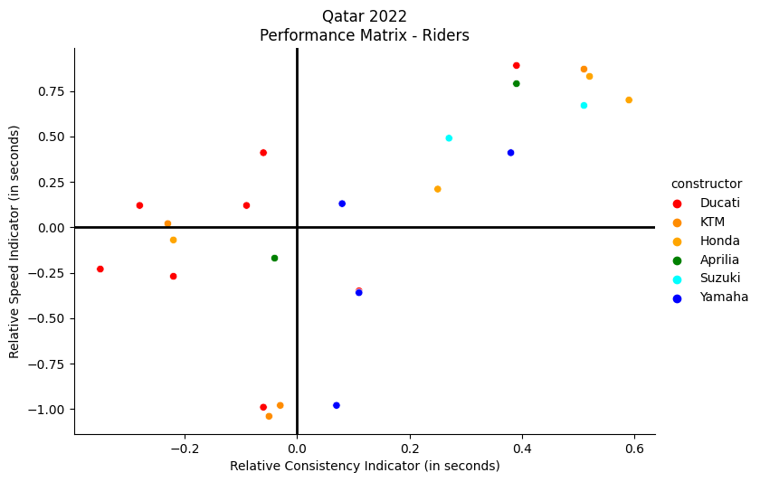

In the case of Qatar, we can see how this graph helps us clearly visualize the struggle of the Ducati teams in having a consistent pace (with the exception of the winner, Bastianini). The Suzuki team had a good overall performance, both in terms of speed and consistency.

sns.relplot(data=performanceITA[performanceITA['performance_index'] > -3], 
            x='pace_consistency_index', 
            y='pace_speed_index', hue='constructor', 
            palette=['red', 'blue', 'green', 'darkorange', 'orange', 'aqua'], 
            # size='points', 
            # sizes=[30, 80], 
            # alpha=0.8, 
            legend='brief', aspect=1.5)

plt.title("Mugello 2022\nPerformance Matrix - Riders")
plt.xlabel("Relative Consistency Indicator (in seconds)")
plt.ylabel("Relative Speed Indicator (in seconds)")

plt.axhline(y=0, color='black', linestyle='-', linewidth=2)
plt.axvline(x=0, color='black', linestyle='-', linewidth=2)

plt.show()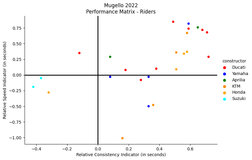

At Mugello, it’s interesting to note how the riders who scored points are all grouped in the upper-right quadrant, which means their values for speed and consistency were above average (confirming the demonstrated relationship between the two variables). Only Quartararo (who finished second) demonstrated both consistency and speed among the Yamaha riders, while the other three Yamahas suffered from a noticeable lack of speed that prevented them from scoring points. The Ducati team had a good overall performance, with most of their riders largely confirming their high performance usually demonstrated at their home circuit.

A performance-based ranking

The two variables quantifying the race pace can be combined to create an index that summarizes a rider’s performance in a single value. We will call this a “performance indicator”: an aggregation of the speed and consistency values of a competitor.

The following table shows the results of the Qatar race along with these indicators. Specifically, from left to right, it includes the starting position, finishing position, difference in positions at the finish, points earned, speed indicator, consistency indicator, and the aggregated performance indicator. This results table, ordered by the latter variable, presents a “revisited” ranking based on the performance demonstrated by the riders regardless of the final result and events of the race.

perfQAT = performanceQAT.drop(columns=[
    'avg_speed', 'avg_laptime', 'delta_avg_laptime',
    'delta_std_laptime']).sort_values('performance_index', ascending=False).reset_index()
perfQAT.index += 1
perfQAT.drop(columns='constructor')

	rider	grid	position	pos_delta	points	pace_speed_index	pace_consistency_index	performance_index
1	Brad Binder	7	2.0	5.0	20	0.87	0.51	0.69
2	Pol Espargaro	6	3.0	3.0	16	0.83	0.52	0.67
3	Enea Bastianini	2	1.0	1.0	25	0.89	0.39	0.64
4	Marc Marquez	3	5.0	-2.0	11	0.70	0.59	0.64
5	Aleix Espargaro	5	4.0	1.0	13	0.79	0.39	0.59
6	Joan Mir	8	6.0	2.0	10	0.67	0.51	0.59
7	Fabio Quartararo	11	9.0	2.0	7	0.41	0.38	0.40
8	Alex Rins	10	7.0	3.0	9	0.49	0.27	0.38
9	Takaaki Nakagami	6	10.0	-4.0	6	0.21	0.25	0.23
10	Johann Zarco	3	8.0	-5.0	8	0.41	-0.06	0.17
11	Franco Morbidelli	12	11.0	1.0	5	0.13	0.08	0.10
12	Francesco Bagnaia	9	NaN	-9.0	0	0.12	-0.09	0.01
13	Jorge Martin	1	NaN	-17.0	0	0.12	-0.28	-0.08
14	Maverick Viñales	9	12.0	-3.0	4	-0.17	-0.04	-0.10
15	Miguel Oliveira	4	NaN	-14.0	0	0.02	-0.23	-0.11
16	Andrea Dovizioso	10	14.0	-4.0	2	-0.36	0.11	-0.12
17	Luca Marini	7	13.0	-6.0	3	-0.35	0.11	-0.12
18	Alex Marquez	8	NaN	-10.0	0	-0.07	-0.22	-0.14
19	Marco Bezzecchi	5	NaN	-13.0	0	-0.27	-0.22	-0.25
20	Jack Miller	4	NaN	-14.0	0	-0.23	-0.35	-0.29
21	Darryn Binder	14	16.0	-2.0	0	-0.98	0.07	-0.45
22	Remy Gardner	12	15.0	-3.0	1	-0.98	-0.03	-0.50
23	Fabio Di Giannantonio	11	17.0	-6.0	0	-0.99	-0.06	-0.53
24	Raul Fernandez	13	18.0	-5.0	0	-1.04	-0.05	-0.55

In this “new” ranking (sorted by the aggregated performance indicator), it is interesting to note that the winner (Enea Bastianini), who dominated the race from the first position since the beginning, is relegated to the third position behind Brad Binder and Pol Espargaro. This is due to the fact that these two riders have shown to have a greater speed and consistency than Enea, who, apart from the victory, has equalled the performance of Marc Marquez.

The same concept is applied to the race performances of the constructors in the following table.

perfQAT_constr = perfQAT.groupby('constructor')[['pace_speed_index', 'pace_consistency_index', 'performance_index']].mean().sort_values('performance_index', ascending=False).round(2)
# perfQAT_constr = perfQAT_constr.sort_values('performance_index', ascending=False).reset_index()
# perfQAT_constr.index += 1
display(perfQAT_constr)

sns.relplot(data=perfQAT_constr, 
            x='pace_consistency_index', 
            y='pace_speed_index', hue='constructor', 
            palette=['aqua', 'orange', 'green', 'blue', 'red', 'darkorange'], 
            # size='points', 
            # sizes=[30, 80], 
            # alpha=0.8, 
            legend='brief', aspect=1.5)

plt.title("Qatar 2022\nPerformance Matrix - Constructors")
plt.xlabel("Relative Consistency Indicator (in seconds)")
plt.ylabel("Relative Speed Indicator (in seconds)")

plt.axhline(y=0, color='black', linestyle='-', linewidth=2)
plt.axvline(x=0, color='black', linestyle='-', linewidth=2)

plt.show()

	pace_speed_index	pace_consistency_index	performance_index
constructor
Suzuki	0.58	0.39	0.48
Honda	0.42	0.28	0.35
Aprilia	0.31	0.18	0.24
Yamaha	-0.20	0.16	-0.02
Ducati	-0.04	-0.07	-0.06
KTM	-0.28	0.05	-0.12

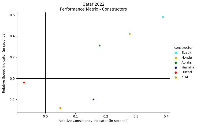
As we can see, thanks in part to the performance matrix applied to the constructors, Suzuki was the most “performant” motorcycle in Qatar 2022, along with Honda and Aprilia. Ducati, Yamaha, and KTM had inferior performances.

Conclusion

For the purpose of providing more technical and structured information to motorsports fans, we have demonstrated in this article how public data can be used to extract important insights on race and competitors performance. While the race results remain undoubtedly the reference for assigning race points, it is still crucial to be able to objectively measure and evaluate the pace of each rider, regardless of the outcome at the checkered flag and all the race events. By examining two MotoGP races in the 2022 season, we first established the importance of visually analyzing the race progression in terms of lap times in order to:

• Examine the overall evolution of tire performance and degradation;
• Compare the lap time evolution of riders, teams, and constructors (also in relation to the race average).

We then demonstrated how lap data can be used to analyze the adaptation of riders, teams, and constructors to different track segments, with the help of aggregate metrics for intermediate sector times.

Finally, we demonstrated the usefulness of quantifying the performances of riders, teams, and constructors through quantitative indicators that take into account relative speed and consistency, the two fundamental variables in a theoretical definition of performance.

In conclusion, the research findings confirm the validity of the initial hypothesis and provide a satisfying answer to the questions that were posed at the beginning of the investigation. It is also believed that this study constitutes an important starting point for the creation of an engaging technical information format for motor racing. The ultimate goal is to promote a constructive and informed debate among industry experts and enthusiasts, providing objective information that allows for statistical evaluation of the performances of riders and vehicles. In this way, we could contribute to fostering a more aware and informed motor racing culture, capable of fully appreciating the technical complexity of this type of sport, especially for those more demanding fans.